Module 2

Classification and Regression

Author

Yike Zhang

Published

August 28, 2025

Class Activities

Week 2

Recap

Link to Google Form

Examples

Example 1: Calculate the Entropy

💡 Using the math library in Python
import math
# probability of class "buy"
p_buy = 0.40

# probability of class "not buy"
p_not_buy = 0.60

# calculate entropy
entropy = -(p_buy * math.log2(p_buy) +
            p_not_buy * math.log2(p_not_buy))

# print out the result
print(entropy)
0.9709505944546686
💡 Using the scikit-learn library in Python
from scipy.stats import entropy
# probability of class "buy"
p_buy = 0.40

# probability of class "not buy"
p_not_buy = 0.60

probabilities = [p_buy, p_not_buy]

# calculate entropy
entropy = entropy(probabilities, base=2)

print(entropy)
0.9709505944546688

Example 2: Use Scikit-learn DecisionTreeClassifier function on the Cat Dataset

import pandas as pd
from sklearn.tree import DecisionTreeClassifier, export_text, plot_tree
import matplotlib.pyplot as plt

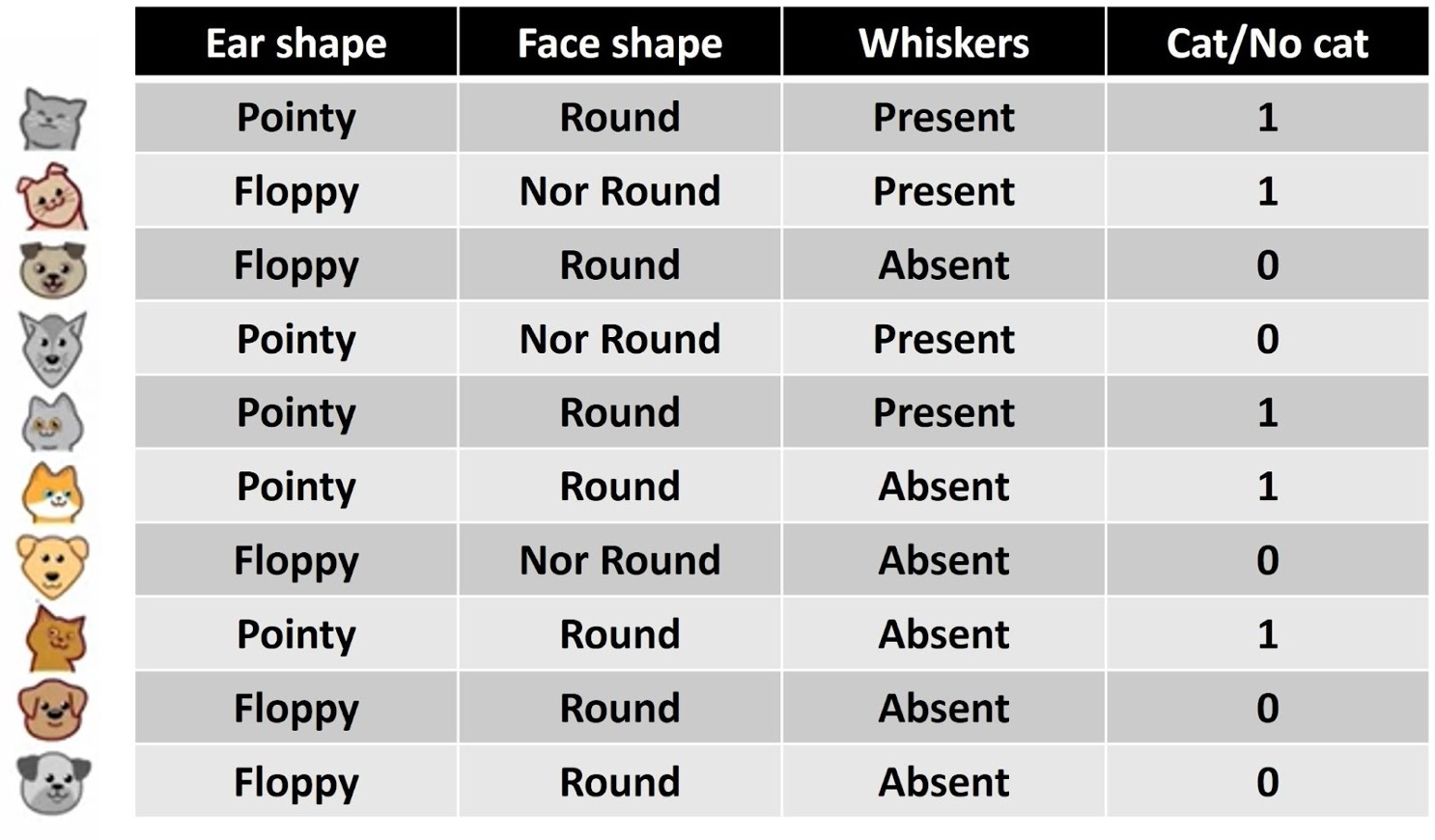
# Load the cat dataset mentioned in class
data = [
    {"Ear shape":"Pointy", "Face shape":"Round",     "Whiskers":"Present", "Cat/No cat":1},
    {"Ear shape":"Floppy", "Face shape":"Not Round", "Whiskers":"Present", "Cat/No cat":1},
    {"Ear shape":"Floppy", "Face shape":"Round",     "Whiskers":"Absent",  "Cat/No cat":0},
    {"Ear shape":"Pointy", "Face shape":"Not Round", "Whiskers":"Present", "Cat/No cat":0},
    {"Ear shape":"Pointy", "Face shape":"Round",     "Whiskers":"Present", "Cat/No cat":1},
    {"Ear shape":"Pointy", "Face shape":"Round",     "Whiskers":"Absent",  "Cat/No cat":1},
    {"Ear shape":"Floppy", "Face shape":"Not Round", "Whiskers":"Absent",  "Cat/No cat":0},
    {"Ear shape":"Pointy", "Face shape":"Round",     "Whiskers":"Absent",  "Cat/No cat":1},
    {"Ear shape":"Floppy", "Face shape":"Round",     "Whiskers":"Absent",  "Cat/No cat":0},
    {"Ear shape":"Floppy", "Face shape":"Round",     "Whiskers":"Absent",  "Cat/No cat":0},
]
df = pd.DataFrame(data)

# Split the dataset into features (X) and target variable (y)
X = pd.get_dummies(df.drop(columns=["Cat/No cat"]))
y = df["Cat/No cat"]

# Train our decision tree (we use entropy for IG in the sklearn library)
# Not limit the depth of the tree (max_depth=None) to allow full growth
clf = DecisionTreeClassifier(criterion="entropy", max_depth=None, random_state=0)
clf.fit(X, y)

# Show decision rules
print("Decision Tree Rules:\n")
print(export_text(clf, feature_names=list(X.columns)))

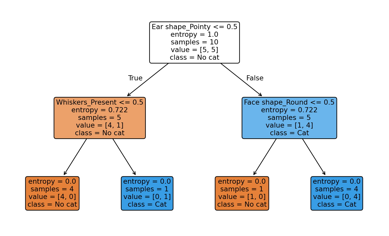
# Plot the tree use the plot_tree function
print("Decision Tree Diagram:\n")
plt.figure(figsize=(10,6))
plot_tree(clf, feature_names=X.columns, class_names=["No cat","Cat"], filled=True, rounded=True)
plt.show()
Decision Tree Rules:

|--- Ear shape_Pointy <= 0.50
|   |--- Whiskers_Present <= 0.50
|   |   |--- class: 0
|   |--- Whiskers_Present >  0.50
|   |   |--- class: 1
|--- Ear shape_Pointy >  0.50
|   |--- Face shape_Round <= 0.50
|   |   |--- class: 0
|   |--- Face shape_Round >  0.50
|   |   |--- class: 1

Decision Tree Diagram:

Example 3: KNN Classifier

The example below uses the KNN Classifier to classify the Iris dataset. We will visualize the decision boundary with different values of k (number of closest neighbors).

import matplotlib.pyplot as plt

from sklearn.inspection import DecisionBoundaryDisplay
from sklearn.neighbors import KNeighborsClassifier
from sklearn.pipeline import Pipeline
from sklearn.preprocessing import StandardScaler
from sklearn.datasets import load_iris
from sklearn.model_selection import train_test_split

iris = load_iris(as_frame=True)
X = iris.data[["sepal length (cm)", "sepal width (cm)"]]
y = iris.target
X_train, X_test, y_train, y_test = train_test_split(X, y, stratify=y, random_state=0)

clf = Pipeline(
    steps=[("scaler", StandardScaler()), ("knn", KNeighborsClassifier(weights="uniform"))]
)

_, axs = plt.subplots(ncols=3, figsize=(12, 5))

for ax, neighbors in zip(axs, (1, 5, 21)):
    clf.set_params(knn__n_neighbors=neighbors).fit(X_train, y_train)
    disp = DecisionBoundaryDisplay.from_estimator(
        clf,
        X_test,
        response_method="predict",
        plot_method="pcolormesh",
        xlabel=iris.feature_names[0],
        ylabel=iris.feature_names[1],
        shading="auto",
        alpha=0.7,
        ax=ax,
    )
    scatter = disp.ax_.scatter(X.iloc[:, 0], X.iloc[:, 1], c=y, edgecolors="k")
    disp.ax_.legend(
        scatter.legend_elements()[0],
        iris.target_names,
        loc="lower left",
        title="Classes",
    )
    _ = disp.ax_.set_title(
        f"3-Class classification\n(k={clf[-1].n_neighbors})"
    )

plt.show()

Example 4: Implementing KNN from Scratch in Python

Given a set of training data points and their corresponding labels, the function knn_predict predicts the label for a new test point based on the majority label of its k-nearest neighbors. We use Counter function from the collections library to find the most common label among the neighbors.

import numpy as np
from collections import Counter

# Defining the Euclidean Distance Function
# euclidean_distance function is to calculate euclidean distance between points.
def euclidean_distance(point1, point2):
    return np.sqrt(np.sum((np.array(point1) - np.array(point2))**2))

def knn_predict(training_data, training_labels, test_point, k):
    distances = []
    for i in range(len(training_data)):
        dist = euclidean_distance(test_point, training_data[i])
        distances.append((dist, training_labels[i]))
    distances.sort(key=lambda x: x[0])
    k_nearest_labels = [label for _, label in distances[:k]]
    return Counter(k_nearest_labels).most_common(1)[0][0]

training_data = [[1, 2], [2, 3], [3, 4], [6, 7], [7, 8]]
training_labels = ['A', 'A', 'A', 'B', 'B']
test_point = [4, 5]
k = 3 # Number of the closest neighbors to consider

prediction = knn_predict(training_data, training_labels, test_point, k)
print(f"The predicted class for the test point is: {prediction}")
The predicted class for the test point is: A

Plot the decision boundary of the KNN classifier implemented from scratch.

Hands-on Practice

Q1: Will you like a movie? Please classify the following movies using Decision Tree Classifier taught in the class.

Movie Type Length IMDb Rating Liked?
m1 Comedy Short 7.2 Yes
m2 Drama Medium 9.3 Yes
m3 Comedy Medium 5.1 No
m4 Drama Long 6.9 No
m5 Drama Medium 8.3 Yes
m6 Drama Short 4.5 No
m7 Comedy Short 8.0 Yes
m8 Drama Medium 7.5 Yes

Q2: Suppose we have height, weight and T-shirt size of some customers and we need to predict the T-shirt size of a new customer given only height and weight information we have. Data including height, weight and T-shirt size information is shown in the table below. New customer named ‘Monica’ has height 161cm and weight 61kg. Can you use KNN Classifier to predict Monica’s T-shirt size? k is set to be 5 in this example.

1 2 3 4 5 6 7 8 9 10 11 12 13 14 15 16 17 18
Height (cms) 158 158 158 160 160 163 163 160 163 165 165 165 168 168 168 170 170 170
Weight (kgs) 58 59 63 59 60 60 61 64 64 61 62 65 62 63 66 63 64 68
T-Shirt Size M M M M M M M L L L L L L L L L L L

Q3 (Optional): Use Decision Tree Classifier to classify the Pokémon Dataset (click the link to download the dataset). Please refer to this YouTube Video to help you get started.

Week 3

Recap

Link to Google Form

Examples

Example 1: SVM Classifier

The example below uses the SVM Classifier to classify the Iris dataset (setosa or versicolor). We will visualize the SVM decision boundary in the plot.

import matplotlib.pyplot as plt
import numpy as np
from sklearn.svm import SVC
from sklearn import datasets

# Load the Iris dataset
iris = datasets.load_iris(as_frame=True)
X = iris.data[["petal length (cm)", "petal width (cm)"]].values
y = iris.target

setosa_or_versicolor = (y == 0) | (y == 1)
X = X[setosa_or_versicolor]
y = y[setosa_or_versicolor]

# Train the SVM Classifier
svm_clf = SVC(kernel="linear", C=1e100) # C is a Regularization Parameter
svm_clf.fit(X, y)

def plot_svc_decision_boundary(svm_clf, xmin, xmax):
    w = svm_clf.coef_[0]
    b = svm_clf.intercept_[0]

    # At the decision boundary, w0*x0 + w1*x1 + b = 0
    # => x1 = -w0/w1 * x0 - b/w1
    x0 = np.linspace(xmin, xmax, 200)
    decision_boundary = -w[0] / w[1] * x0 - b / w[1]

    margin = 1/w[1]
    gutter_up = decision_boundary + margin
    gutter_down = decision_boundary - margin
    svs = svm_clf.support_vectors_

    plt.plot(x0, decision_boundary, "k-", linewidth=2, zorder=-2)
    plt.plot(x0, gutter_up, "k--", linewidth=2, zorder=-2)
    plt.plot(x0, gutter_down, "k--", linewidth=2, zorder=-2)
    plt.scatter(svs[:, 0], svs[:, 1], s=180, facecolors='#AAA',
                zorder=-1)

fig, axes = plt.subplots(ncols=1, figsize=(10, 2.7), sharey=True)
plot_svc_decision_boundary(svm_clf, 0, 5.5)
plt.plot(X[:, 0][y==1], X[:, 1][y==1], "bs")
plt.plot(X[:, 0][y==0], X[:, 1][y==0], "yo")
plt.xlabel("Petal length")
plt.axis([0, 5.5, 0, 2])
plt.gca().set_aspect("equal")
plt.grid()
plt.show()

Hands-on Practice

Q1: Consider the car theft problem with attributes Color, Type, Origin, and the target, Stolen can be either Yes or No. Please Use the Naive Bayes Classifier to solve the following problems.

Car Theft Problem
Example No. Color Type Origin Stolen?
1 Red Sports Domestic Yes
2 Red Sports Domestic No
3 Red Sports Domestic Yes
4 Yellow Sports Domestic No
5 Yellow Sports Imported Yes
6 Yellow SUV Imported No
7 Yellow SUV Imported Yes
8 Yellow SUV Domestic No
9 Red SUV Imported No
10 Red Sports Imported Yes

Q1.1: What is the possibilty of a Red SUV Domestic car being stolen?

Q1.2: What is the possibilty of a Red SUV Domestic car Not being stolen?

Q1.3: Given the possibilites, do you think the Red SUV Domestic car will be stolen or not?

Q2: Could you use Support Vector Machine (SVM) to predict a Pulsar Star? The dataset can be downloaded here. Pulsars are a rare type of Neutron star that produce radio emission detectable here on Earth. They are of considerable scientific interest as probes of space-time, the inter-stellar medium, and states of matter. Classification algorithms in particular are being adopted, which treat the data sets as binary classification problems. Here the legitimate pulsar examples form minority positive class and spurious examples form the majority negative class. The dataset here contains 16,259 spurious examples caused by RFI/noise, and 1,639 real pulsar examples. Each row lists the variables first, and the class label is the final entry. The class labels used are 0 (negative) and 1 (positive).

Attribute Information: Each candidate is described by 8 continuous variables, and a single class variable. The first four are simple statistics obtained from the integrated pulse profile. The remaining four variables are similarly obtained from the DM-SNR curve . These are summarised below:

  1. Mean of the integrated profile.
  2. Standard deviation of the integrated profile.
  3. Excess kurtosis of the integrated profile.
  4. Skewness of the integrated profile.
  5. Mean of the DM-SNR curve.
  6. Standard deviation of the DM-SNR curve.
  7. Excess kurtosis of the DM-SNR curve.
  8. Skewness of the DM-SNR curve.
  9. Class

Example code is provided below for references (contain data preprocessing). The code below only prepares the data. You need to add code for SVM model training and prediction after the data preparation part. We aim to run SVM with default hyperparameters. The model prediction accuracy should be 0.9827 at the end. Note that if you do not have a Python IDE set up, you can run the following code in Google Colab.

import numpy as np # linear algebra
import pandas as pd # data processing, CSV file I/O (e.g. pd.read_csv)
from sklearn.model_selection import train_test_split # Split the dataset into training and testing sets
from sklearn.preprocessing import StandardScaler # Feature scaling

df = pd.read_csv("pulsar_stars.csv")
print(f"Dataset shape: {df.shape}")

# let's preview the dataset
# print(df.head(5))

print(f"Column names: {df.columns.str.strip()}")

# view summary of dataset
# print(f"Dataset summary:\n{df.describe()}")

X = df.drop(['target_class'], axis=1) # Drop specified labels from rows or columns.
y = df['target_class']

X_train, X_test, y_train, y_test = train_test_split(X, y, test_size = 0.2, random_state = 0)

print(f"Training set shape: {X_train.shape}, Test set shape: {X_test.shape}")

# Feature Scaling
scaler = StandardScaler()
X_train = scaler.fit_transform(X_train)
X_test = scaler.transform(X_test)

# Construct DataFrames
X_train = pd.DataFrame(X_train, columns=X.columns)
X_test = pd.DataFrame(X_test, columns=X.columns)

# After data preparation, we now run SVM with default hyperparameters
# Code for SVM model training and evaluation goes below ⬇️
Dataset shape: (17898, 9)
Column names: Index(['Mean of the integrated profile',
       'Standard deviation of the integrated profile',
       'Excess kurtosis of the integrated profile',
       'Skewness of the integrated profile', 'Mean of the DM-SNR curve',
       'Standard deviation of the DM-SNR curve',
       'Excess kurtosis of the DM-SNR curve', 'Skewness of the DM-SNR curve',
       'target_class'],
      dtype='object')
Training set shape: (14318, 8), Test set shape: (3580, 8)

Week 4

Recap

Link to Google Form

Examples

Release Soon

Hands-on Practice

Release Soon