Module 4

Neural Networks

Class Activities

Week 8

Recap

Link to Google Form

Examples

Example 1: Perceptron Animation

In this example, we will implement the Perceptron algorithm from scratch using Python and NumPy. We will visualize the training process by using an animated GIF that shows how the decision boundary evolves as the model learns from the data. That hollow circle is just a visual highlight for the current training sample in that frame. It doesn’t affect the model as it’s there so you can see which point the perceptron just “looked at” or “refers to” when updating the weights and shifting the decision boundary. This following example is modified from here, and the toy dataset can be found here.

import numpy as np
import matplotlib.pyplot as plt

# Prepare the dataset
data = np.genfromtxt('perceptron_toydata.txt', delimiter='\t')
X, y = data[:, :2], data[:, 2]
y = y.astype(np.int32)

# Shuffle and split the dataset
shuffle_idx = np.arange(y.shape[0])
shuffle_rng = np.random.RandomState(123)
shuffle_rng.shuffle(shuffle_idx)
X, y = X[shuffle_idx], y[shuffle_idx]

# Define the Perceptron model
class Perceptron():
    def __init__(self, num_features):
        self.num_features = num_features
        self.learning_rate = 1.0
        self.weights = np.zeros((num_features, 1), dtype=np.float32)
        self.bias = np.zeros(1, dtype=np.float32)

    def forward(self, x):
        linear = np.dot(x, self.weights) + self.bias
        predictions = np.where(linear > 0., 1, 0)
        return predictions
        
    def backward(self, x, y):  
        predictions = self.forward(x)
        errors = y - predictions
        return errors
        
    def train(self, x, y, epochs):
        for e in range(epochs):
            for i in range(y.shape[0]):
                errors = self.backward(x[i].reshape(1, self.num_features), y[i]).reshape(-1)
                self.weights += self.learning_rate * (errors * x[i]).reshape(self.num_features, 1)
                self.bias += self.learning_rate * errors
                
    def evaluate(self, x, y):
        predictions = self.forward(x).reshape(-1)
        accuracy = np.sum(predictions == y) / y.shape[0]
        return accuracy

# Train the Perceptron model and store weights and biases for each step
all_weights = []
all_biases = []
ppn = Perceptron(num_features=2)
acc = 0
for epoch in range(10):
    for i in range(X.shape[0]):
        all_weights.append(ppn.weights.copy())
        all_biases.append(ppn.bias.copy())
        ppn.train(X[i].reshape(1, -1), y[i].reshape(-1), epochs=1)
        acc = ppn.evaluate(X, y)
        if acc == 1.0: break
    if acc == 1.0:
        all_weights.append(ppn.weights.copy())
        all_biases.append(ppn.bias.copy())
        break

Example 2: Implementation of Adaline Linear Neuron in Numpy

In this example, we will implement the Adaline (Adaptive Linear Neuron) algorithm from scratch using Python and NumPy. We will use the classic Iris dataset for training and testing the model. This following example is modified from here.

import numpy as np
import matplotlib.pyplot as plt
from sklearn.datasets import load_iris
from sklearn.model_selection import train_test_split

# Load the Iris dataset
iris = load_iris()
X = iris.data[:, [0, 2]] # Use only two features for simplicity
y = iris.target
y = np.where(y == 0, -1, 1)

# Split the dataset into training and testing sets
X_train, X_test, y_train, y_test = train_test_split(X, y, test_size=0.4, random_state=1)

# Standardize the features
X_train_std = (X_train - X_train.mean()) / X_train.std()
X_test_std = (X_test - X_train.mean()) / X_train.std()

# Define the Adaline Model
class Adaline:
    def __init__(self, learning_rate=0.01, n_iter=50):
        self.learning_rate = learning_rate
        self.n_iter = n_iter

    def fit(self, X, y):
        n_samples, n_features = X.shape
        self.weights = np.zeros(n_features)
        self.bias = 0
        self.cost_ = []
        for _ in range(self.n_iter):
            y_pred = self.activation(X)
            error = y - y_pred
            self.weights += self.learning_rate * np.dot(X.T, error) # Update weights
            self.bias += self.learning_rate * np.sum(error) # Update bias
            cost = 0.5 * np.sum(error ** 2)
            self.cost_.append(cost)

    def activation(self, X):
        return np.dot(X, self.weights) + self.bias

    def predict(self, X):
        return np.where(self.activation(X) >= 0.0, 1, -1)

# Train the Adaline model
adaline_model = Adaline(learning_rate=0.001, n_iter=80)
adaline_model.fit(X_train_std, y_train)

# Plot the cost over epochs
plt.plot(range(1, len(adaline_model.cost_) + 1), adaline_model.cost_, marker='o')
plt.xlabel('Epochs')
plt.ylabel('Sum of Squared Errors')
plt.title('Adaline Training Curve')
plt.show()

# Evaluate the Adaline model
y_pred = adaline_model.predict(X_test_std)
accuracy = np.sum(y_test == y_pred) / len(y_test)
print("Accuracy:", accuracy)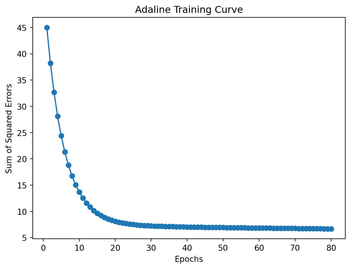

Accuracy: 0.9833333333333333

Hands-on Practice

Q1: Please use the Perceptron algorithm from scikit-learn library to train the Iris dataset.

from sklearn.datasets import load_iris
from sklearn.model_selection import train_test_split

# Load the Iris dataset
data = load_iris()

# Splitting the dataset to train data and test data
X, y = data.data[:100, :], data.target[:100]
X_train, X_test, y_train, y_test = train_test_split(X, y, test_size=0.2, random_state=42)

# Please write your code below this line

Accuracy: 1.0

Q2: Comparing the Adaline and Perceptron model performance on the following synthetic dataset.

import numpy as np
import pandas as pd
import matplotlib.pyplot as plt
from sklearn.datasets import make_classification
import matplotlib.pyplot as plt

from sklearn.datasets import make_classification
import matplotlib.pyplot as plt

# Generate a synthetic binary classification dataset
X, y = make_classification(
    n_samples=4000,
    n_features=2,
    n_informative=2,
    n_redundant=0,
    random_state=42,
)

# Plot the generated data points
plt.figure(figsize=(8, 6))
plt.scatter(X[:, 0], X[:, 1], marker='o', c=y, edgecolor='k', alpha=0.6)
plt.xlabel("Feature 1")
plt.ylabel("Feature 2")
plt.title("Dataset")
plt.show()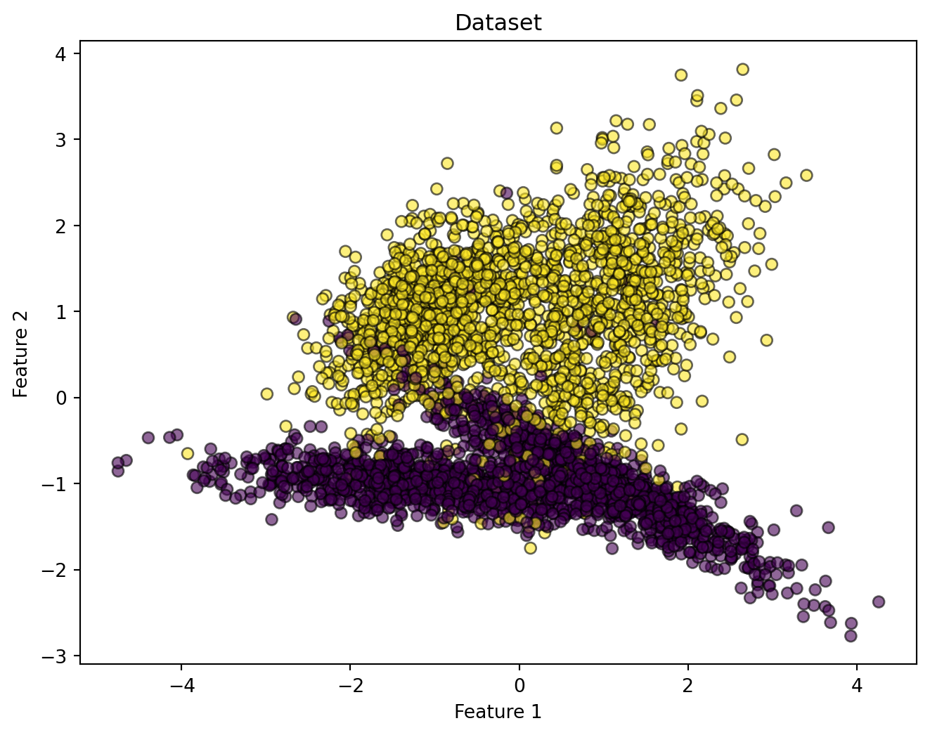

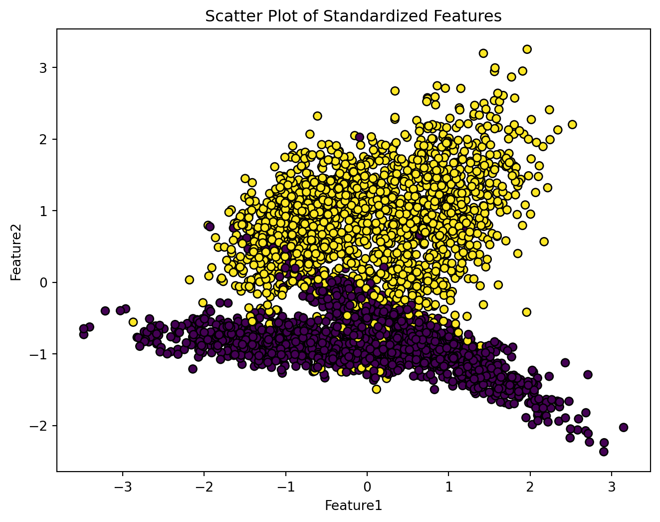
Q2.1: Please standardize the above dataset and store the standardized features in variable X. Afterwards, plot the standardized dataset as showing in the following.

Q2.2: Please split the data into training set and testing set with 80% training data and 20% testing data. Use random state 42 for reproducibility.

# Please write your code below this line
# Split the dataset into training and testing sets

Training set size: 3200 samples
Testing set size: 800 samples

Q2.3: Please implement a Perceptron learning algorithm on the standardized dataset. In this example, we set the learning rate to 0.002 and the number of iterations to 400. You may adjust these two parameters to see how they affect the performance of the model. After training the model, please plot the decision boundary of the Perceptron model.

# Please write your code below this line
# Perceptron model implementation and visualization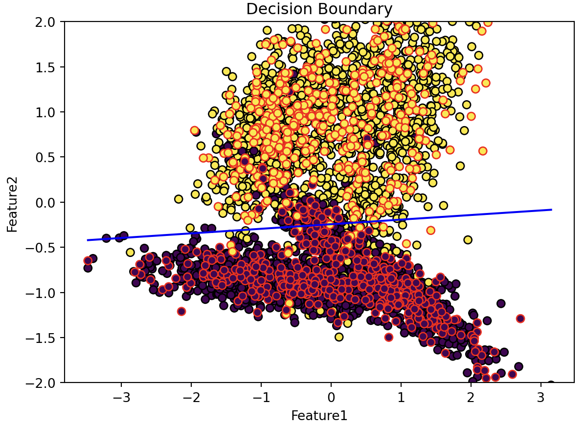

Q2.4: Please implement an Adaline learning algorithm on the standardized dataset. In this example, we set the learning rate to 0.001 and the number of iterations to 400. You may adjust these two parameters to see how they affect the performance of the model. After training the model, please plot the decision boundary of the Adaline model.

# Please write your code below this line
# Adaline model implementation and visualization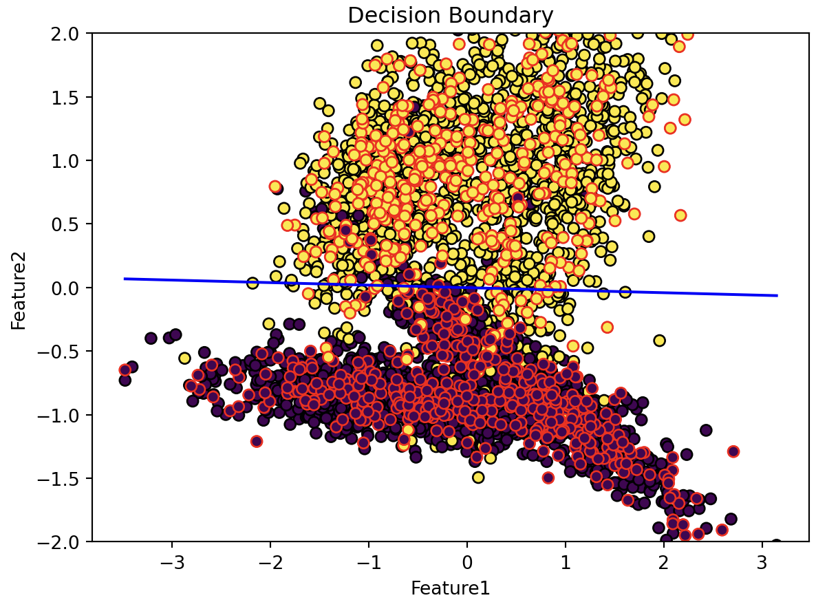

Q2.4: Comparing the accuracy of Adaline and Perceptron using Bar Graph from the matplotlib library.

# Please write your code below this line
# Adaline model implementation and visualization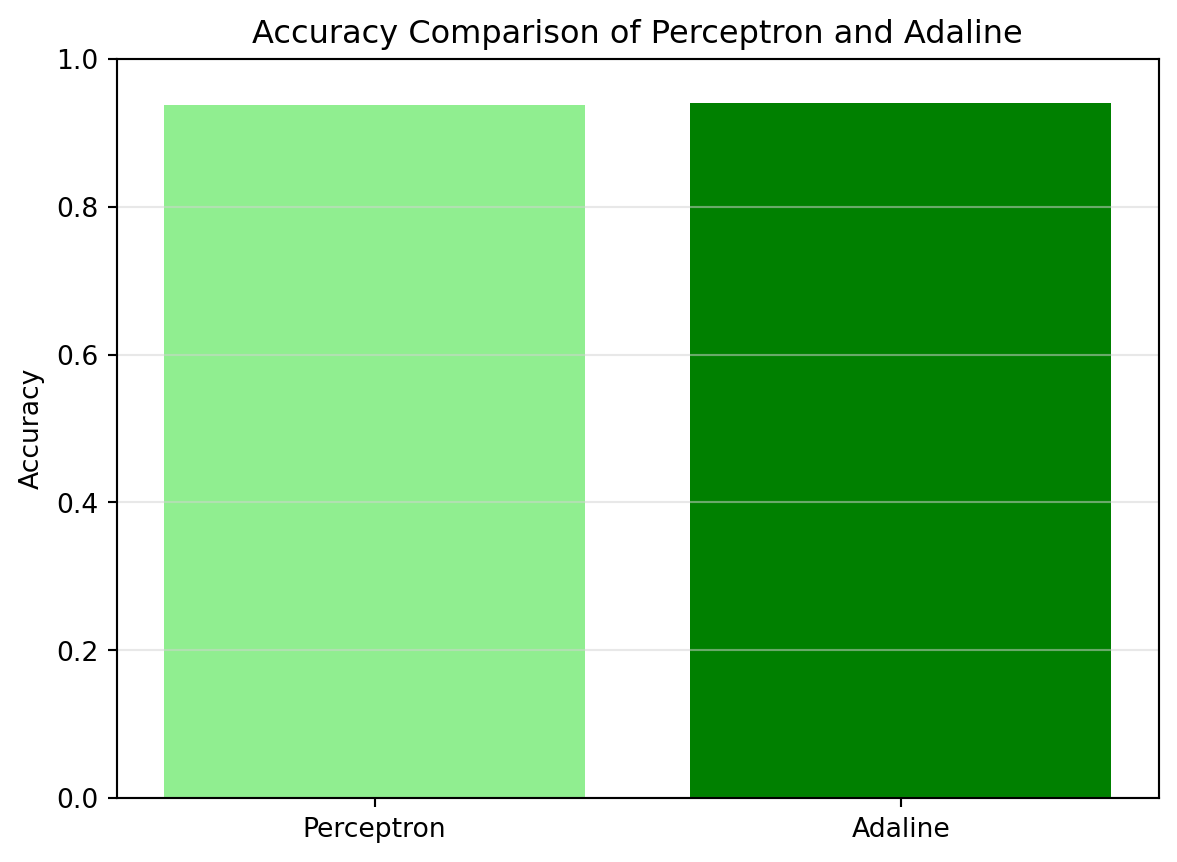

Please note that Q2 is adopted and modified from a kaggle example, and you may find more detailed explaination from the provided link.

Week 9

Recap

Link to Google Form

Examples

Example 1: Neural Network Forward Propagation

In this example, we will implement a simple feedforward neural network using NumPy and the following code is adopted and modified from here.

import numpy as np
import pandas as pd

data = {'cgpa': [8.5, 9.2, 7.8], 'profile_score': [85, 92, 78], 'lpa': [10, 12, 8]}
df = pd.DataFrame(data)
X = df[['cgpa', 'profile_score']].values

def initialize_parameters():
    np.random.seed(1)
    W = np.random.randn(2, 1) * 0.01
    b = np.zeros((1, 1))
    return W, b

def forward_propagation(X, W, b):
    # Linear transformation
    Z = np.dot(X, W) + b
    # Sigmoid activation function
    A = 1 / (1 + np.exp(-Z))  
    return A

W, b = initialize_parameters()
A = forward_propagation(X, W, b)
print("Final Output:\n", A)

Final Output:
 [[0.40566303]
 [0.39810287]
 [0.41326819]]

Example 2: Neural Network Backward Propagation

In this example, we will implement the backward propagation process for a simple feedforward neural network using NumPy, and the following code is adopted and modified from here.

import numpy as np

class NeuralNetwork:
    def __init__(self, input_size, hidden_size, output_size):
        self.input_size = input_size
        self.hidden_size = hidden_size
        self.output_size = output_size

        self.weights_input_hidden = np.random.randn(self.input_size, self.hidden_size)
        self.weights_hidden_output = np.random.randn(self.hidden_size, self.output_size)

        self.bias_hidden = np.zeros((1, self.hidden_size))
        self.bias_output = np.zeros((1, self.output_size))

    def sigmoid(self, x):
        return 1 / (1 + np.exp(-x))

    def sigmoid_derivative(self, x):
        return x * (1 - x)

    def feedforward(self, X):
        self.hidden_activation = np.dot(X, self.weights_input_hidden) + self.bias_hidden
        self.hidden_output = self.sigmoid(self.hidden_activation)

        self.output_activation = np.dot(self.hidden_output, self.weights_hidden_output) + self.bias_output
        self.predicted_output = self.sigmoid(self.output_activation)

        return self.predicted_output

    def backward(self, X, y, learning_rate):
        output_error = y - self.predicted_output
        output_delta = output_error * self.sigmoid_derivative(self.predicted_output)

        hidden_error = np.dot(output_delta, self.weights_hidden_output.T)
        hidden_delta = hidden_error * self.sigmoid_derivative(self.hidden_output)

        self.weights_hidden_output += np.dot(self.hidden_output.T, output_delta) * learning_rate
        self.bias_output += np.sum(output_delta, axis=0, keepdims=True) * learning_rate
        self.weights_input_hidden += np.dot(X.T, hidden_delta) * learning_rate
        self.bias_hidden += np.sum(hidden_delta, axis=0, keepdims=True) * learning_rate

    def train(self, X, y, epochs, learning_rate):
        for epoch in range(epochs):
            output = self.feedforward(X)
            self.backward(X, y, learning_rate)
            if epoch % 4000 == 0:
                loss = np.mean(np.square(y - output))
                print(f"Epoch {epoch}, Loss:{loss}")

# Sample dataset for XOR problem
X = np.array([[0, 0], [0, 1], [1, 0], [1, 1]])

# Target output for the XOR problem
y = np.array([[0], [1], [1], [0]])

# Initialize and Train the Neural Network
nn = NeuralNetwork(input_size=2, hidden_size=4, output_size=1)
nn.train(X, y, epochs=10000, learning_rate=0.1)
output = nn.feedforward(X)
print("Final Predictions after Training:")
print(output)

Epoch 0, Loss:0.2587210173837184
Epoch 4000, Loss:0.015890565252111584
Epoch 8000, Loss:0.0033627357847841152
Final Predictions after Training:
[[0.03969706]
 [0.96741739]
 [0.93734394]
 [0.05146935]]

Example 3: Building Micrograd

Please refer to this amazing video and code by Andrej Karpathy for building Micrograd.

Hands-on Practice

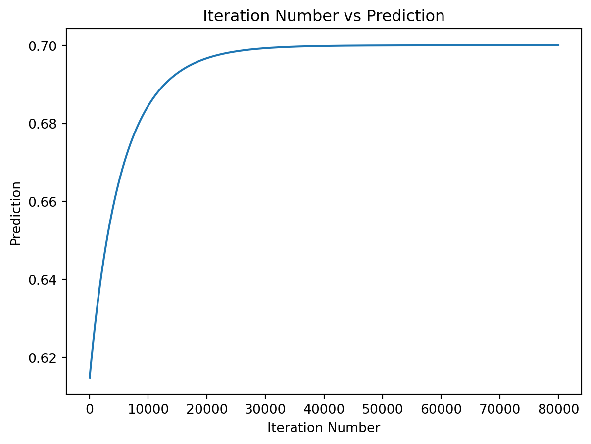
Q1: Coding forward and backward pass in Python. Given the following inputs, weights, and target output, please implement the forward pass to compute the predicted output and the backward pass to update the weights using gradient descent. It is recommended to run for 80000 iterations in this example; however, you may adjust the number of iterations and learning rate to see how they affect the performance of the model. After training the model, please plot the error and predicted output given input x = [0.1, 0.4] over iterations and you should observe that the final prediction result is close to the target value y = 0.7.

import numpy
import matplotlib.pyplot as plt

def sigmoid(sop):
    return 1.0/(1+numpy.exp(-1*sop))

def error(predicted, target):
    return numpy.power(predicted-target, 2)

def error_predicted_deriv(predicted, target):
    return 2*(predicted-target)

def sigmoid_sop_deriv(sop):
    return sigmoid(sop)*(1.0-sigmoid(sop))

def sop_w_deriv(x):
    return x

def update_w(w, grad, learning_rate):
    return w - learning_rate*grad

x1=0.1
x2=0.4

target = 0.7
learning_rate = 0.01

w1=numpy.random.rand()
w2=numpy.random.rand()

predicted_output = []
network_error = []

# Please write your code below this line
# Include forward pass and backward pass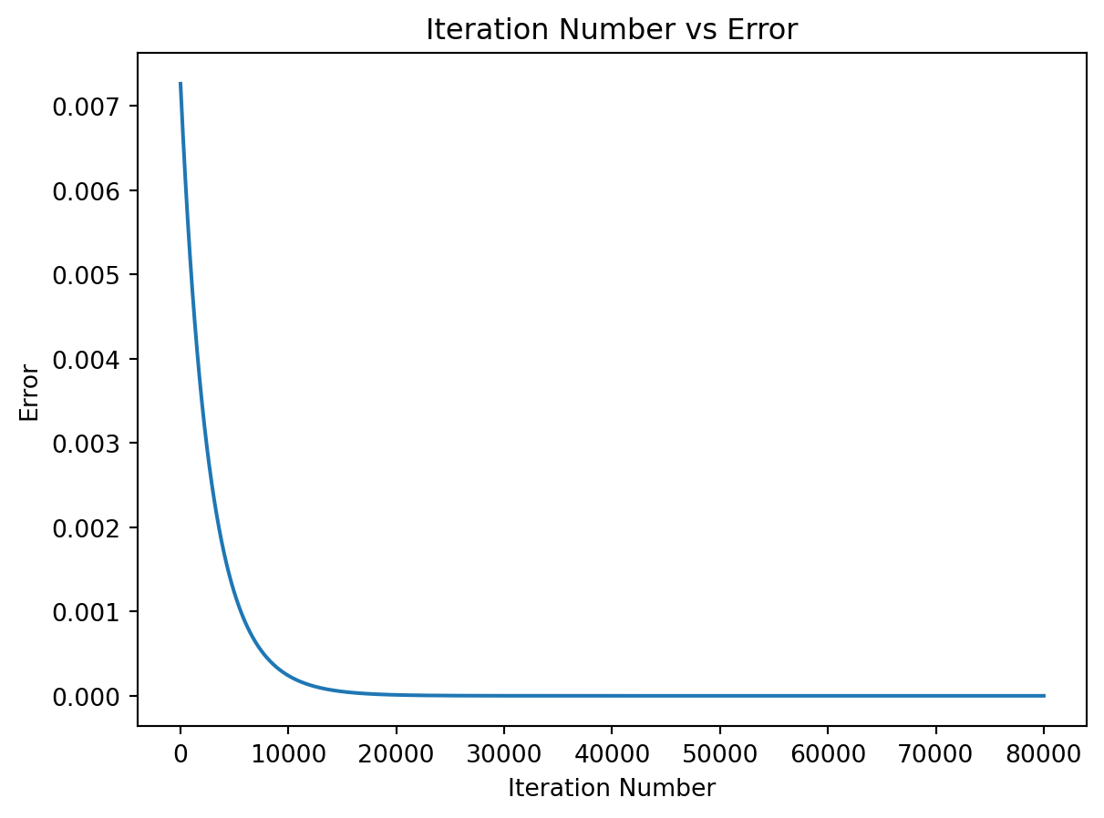

Q2: The following is an example that builds a network with 3 inputs and 1 output. Please use the scikit-learn library to implement the MLPRegressor network. The MLPRegressor model configurations are given below. After training the model, please predict the output given the original input x = [0.1, 0.4, 4.1]. The final prediction result should be close to the target value y = 0.2.

import numpy as np
import matplotlib.pyplot as plt
from sklearn.neural_network import MLPRegressor

# Prepare the dataset
x = np.array([0.1, 0.4, 4.1]).reshape(1, -1) # shape (1, 3)
y = np.array([0.2]).ravel() # shape (1,)          

# Define the Scikit-learn MLPRegressor model
mlp = MLPRegressor(
    hidden_layer_sizes=(7, 5, 4),
    activation="logistic",
    solver="sgd",
    learning_rate="constant",
    learning_rate_init=0.05,
    momentum=0.9,
    max_iter=1,
    warm_start=True,
    random_state=42,
)

# Parameters setting for the MLPRegressor
mlp = MLPRegressor(
    hidden_layer_sizes=(7,5,4),
    activation="logistic",
    solver="sgd",
    learning_rate="constant",
    learning_rate_init=0.05,
    momentum=0.9,
    max_iter=500,
    tol=1e-6,
    n_iter_no_change=20,
    random_state=42,
)

# Please write your code below this line
# Predict the output given the input x

Final Prediction: [0.20030034]
Target Value: [0.2]

Please note that Q1 and Q2 are adopted and modified from this website, and you may find more detailed explaination from the provided link.